
Decision science is a collection of quantitative techniques applied to decision making at both the individual and organizational levels. Its sub-fields include decision analysis, risk analysis, cost-benefit analysis, behavioral decision theory, and more. Decision science takes from both math and psychology to better understand and evaluate decision making.
This three-part series applies decision science to football through decision trees, decision making under uncertainty, and multi-criteria decision making. In this article, we will highlight various tools and methods from decision science and how they can connect to common aspects of football.
"Decision Analysis will not solve a decision problem, nor is it intended to. Its purpose is to produce insight and promote creativity to help decision makers make better decisions."-Ralph Keeney
Decisions often include sequential decisions, major uncertainties, and significant outcomes. It is this complex structure that makes decisions difficult but also exactly where decision analysis can help. First, decision analysis can decompose a decision problem into a set of smaller (hopefully easier to manage) problems before integrating them into a unified course of action.
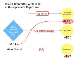
Decision trees are one of the most commonly used tools from the decision analysis toolbox. Note this does not refer to tree-based classification and regression models from the fields of statistics and machine learning. Below is an example of a decision tree that contains one decision opportunity and three events whose outcomes are uncertain. This is a simplification of the well-known problem that offensive coordinators face often: What do we do on 4th down?

The blue diamond is what is known as a Decision Node, where the decision maker (in our example, the coach) gets to make a choice. The yellow circles are Uncertainty Nodes where different outcomes are possible; these are also referred to as Chance Nodes. We consider the outcomes in green as positive (getting a first down or scoring points), while those shown in light red (where the opponent gets the ball) are negative outcomes.
This is, of course, a simplification used for illustrative purposes, but more nuances can be added to the nodes. For instance, is the punt (or the field goal) blocked? What is the probability of a particular field goal kicker making a 55-yard (38-yard line plus 17 yards to account for the end zone and spot of the kick) field goal given the current wind and precipitation conditions? This simplified example is meant to establish a working understanding of decision trees.
However, decision trees also often incorporate the probability of various outcomes of each chance node. Focusing in on the “Is it good?” node associated with the field goal attempt, the probability of making it could be quite high (e.g., Justin Tucker in Allegiant Stadium) or low (e.g., a struggling kicker at Lambeau Field on a very windy December night.)

Additionally, it is important to quantify the payoffs (outcomes shown in the green and light red boxes) on a common scale. As shown thus far, trying to compare scoring three points versus giving up the ball (and getting zero points) is difficult. Giving up the ball is actually worse than getting zero points because the opponent now has the ball and an opportunity to score. So, we need a way to put the situation at the start (or end) of a play on a common scale.
Expected Points (EP) is a quantification of the number of points expected to be scored by the team with the ball before the end of the current drive accounting for factors including the down, distance to go, field position, home-field advantage, and time remaining. Expected Points Added (EPA) is the difference between a team’s Expected Points at the end of a play and their Expected Points at the beginning of a play.
Let’s say that your team (with the struggling kicker, on a very windy December day in Lambeau Field) is down by 1 with 5 minutes to go in the game and facing a 4th and 3 situation at the opponent’s 41-yard line.

In this instance, if you attempt the field goal and make it, the EPA is +2.04. Should you miss it, it is -2.54. This negative stems from both the failure to add points and turning over the ball to your opponent.
Similarly, we calculate the EPA for each of the other possible outcomes on this 4th and 3 as shown in the revised tree below. It may seem counterintuitive that going for (and getting) the first down is worth a larger increase in EPA than kicking the field goal and potentially securing points on that play. However, consider that you still have an opportunity to score a touchdown; if you kick the field goal you do not.
Either negative outcome resulting in a turnover on downs has the same value within the value of a yard or two. Both outcomes of punting are negative, though successfully downing the ball or tackling the returner at the average 15-yard line is noticeably better than kicking it into the end zone for a touchback. Also, notice that NFL punters rarely (maybe 1% of the time) kick the ball into the endzone from this distance.

To “solve” the decision tree, you roll it back from the right to the left, using the so-called “method of backward induction” using the idea of expected value, which is effectively a weighted average. We denote the expected value of an event as E(Event). For example, regarding the field goal, the expected value of attempting the field goal is as follows:
E(Attempted Field Goal) = P(make) x (EPA make) + P(miss) x (EPA miss)
= (.03) x (2.04) + (0.7) x (-2.54)
= -1.16
Using the same procedure E(Go For It) = (0.5)(2.13) + (0.5)(-2.50) = -0.18 and E(Punt) = (0.01)(-1.82) + (0.99)(-1.20) = -1.21 resulting in the following decision tree that has now been “rolled back” by one level.

So, when comparing them at the decision node, the task is to select the choice with the highest expected value. Even though all of them are negative (because your drive may stall), since -0.18 > -0.63 > -1.18, the choice that maximizes the expected value (in terms of expected points added) is to go for the first down.
Note that if the probabilities were different (e.g., you had a strong kicker who consistently hits 50+ yard field goals), the result could have been different. The option of attempting the field goal would certainly be a better choice than punting, and maybe even a better option than going for it. We would have to assess the probability and recalculate.
With this familiar example, we have introduced the idea of expected value and how to use it in decision trees to structure and make decisions. In the next two parts of this three-part series, we will take a look at decision making under uncertainty and what to do when there are multiple objectives and attributes to consider in making a decision.


